In order to accomplish this goal, the first step is to gather data from rcsb.org. That site contains downloadable PDB structures of experiments in various formats.

Although data is stored in multiple formats, in this example, only the formatted fixed-space delimited textual format (PDB) will be used. An alternative to the PDB textual format is its XML version, PDBML, but it sometimes contains malformed atom position naming entries, which can cause problems for data analysis. The older mmCIF and other formats may also be available, but they will not be explained in this article.

The PDB Format

The PDB format is a fragmented fixed-width textual format which can easily be parsed by SQL queries, Java plugins, or Perl modules, for example. Each data type in the file container is represented as a line beginning with the appropriate tag—we’ll go through each tag type in the following subsections. The line length is less than or equal to 80 characters, where a tag takes six or less characters plus one or more spaces which together take eight bytes. There are also cases without spaces between tags and data, usually for CONECT tags.

TITLE

The TITLE tag marks a line as being (part of) the title of the experiment, containing the molecule name and other relevant data like the insertion, mutation, or deletion of a specific amino acid.

12345678901234567890123456789012345678901234567890123456789012345678901234567890

TITLE     A TWO DISULFIDE DERIVATIVE OF CHARYBDOTOXIN WITH DISULFIDE            

TITLE    2 13-33 REPLACED BY TWO ALPHA-AMINOBUTYRIC ACIDS, NMR, 30              

TITLE    3 STRUCTURES                                                           

In the case where there are multiple lines to a TITLE record, then the title has to be concatenated, ordering by a continuation number, which is placed, right-aligned, on bytes 9 and 10 (depending on the number of these lines).

ATOM

The data stored in ATOM lines is coordinate data for each atom in an experiment. Sometimes an experiment has insertions, mutations, alternate locations, or multiple models. This results in repeating the same atom multiple times. Choosing the right atoms will be explained later.

12345678901234567890123456789012345678901234567890123456789012345678901234567890

ATOM    390  N   GLY A  26      -1.120  -2.842   4.624  1.00  0.00           N  

ATOM    391  CA  GLY A  26      -0.334  -2.509   3.469  1.00  0.00           C  

ATOM    392  C   GLY A  26       0.682  -1.548   3.972  1.00  0.00           C  

ATOM    393  O   GLY A  26       0.420  -0.786   4.898  1.00  0.00           O  

ATOM    394  H   GLY A  26      -0.832  -2.438   5.489  1.00  0.00           H  

ATOM    395  HA2 GLY A  26       0.163  -3.399   3.111  1.00  0.00           H  

ATOM    396  HA3 GLY A  26      -0.955  -2.006   2.739  1.00  0.00           H  

The example above is taken from the experiment 1BAH. The first column marks the type of record, and the second column is the serial number of the atom. Every atom in a structure has its own serial number.

Next to the serial number there is the atom position label, which takes four bytes. From that atom position, it is possible to extract the chemical symbol of the element, which is not always present in the record data in its own separate column.

After the atom name there is a three-letter residue code. In the case of proteins, that residue corresponds to an amino acid. Next, the chain is coded with one letter. By chain we mean a single chain of amino acids, with or without gaps, although sometimes ligands can be assigned to a chain; this case is detectable through very large gaps in an amino acid sequence, which is in the next column. Sometimes the same structure can be scanned with mutations included, in which case the insertion code is available in an extra column after the sequence column. The insertion code contains a letter to help to distinguish which residue is affected.

The next three columns are the spatial coordinates of each atom, measured in Angstroms (Å). Next to these coordinates is the occupancy column, which says what the probability is for the atom to be in that place, on the usual scale of zero to one.

The second-last column is the temperature factor, which carries information about the disorder in the crystal, measured in Ų. A value greater than 60Ų signifies disorder, while one lower than 30Ų signifies confidence. It is not always present in PDB files because it depends on the experimental method.

The next columns—symbol and charge—are usually missing. The chemical symbol can be gathered from the atom position column, as we mentioned above. When the charge is present, it’s suffixed to the symbol as an integer followed by + or -, e.g. N1+.

TER

This marks the end of the chain. Even without this line, it is easy to distinguish where a chain ends. Thus, often the TER line is missing.

MODEL and ENDMDL

A MODEL line marks where the model of a structure starts, and it contains the serial number of the model.

After all atomic lines in that model, it ends with an ENDMDL line.

SSBOND

These lines contain disulphide bonds between cysteine amino acids. Disulfide bonds can be present in other residue types, but in this article only amino acids will be analyzed, so only cysteine is included. The following example is from the experiment with code 132L:

12345678901234567890123456789012345678901234567890123456789012345678901234567890

SSBOND   1 CYS A    6    CYS A  127                          1555   1555  2.01

SSBOND   2 CYS A   30    CYS A  115                          1555   1555  2.05

SSBOND   3 CYS A   64    CYS A   80                          1555   1555  2.02

SSBOND   4 CYS A   76    CYS A   94                          1555   1555  2.02

In this example there are four disulfide bonds tagged in the file with their sequence number in the second column. All of these bonds use cysteine (columns 3 and 6), and all of them are present in chain A (columns 4 and 7). After each chain there is a residue sequence number indicating the bond’s position in the peptide chain. Insertion codes are next to each residue sequence, but in this example they aren’t present because there was no amino acid inserted in that region. The two columns before the last one are reserved for symmetry operations, and the last column is the distance between sulfur atoms, measured in Å.

Let’s take a moment to give some context to this data.

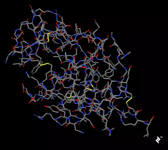
The pictures below, taken using the rcsb.org NGL viewer, show the structure of experiment 132L. In particular, they show a protein without ligands. The first picture uses a stick representation, with CPK coloring showing sulfurs and their bonds in yellow. V-shaped sulfur connections represent methionine connections, while the Z-shaped connections are disulfide bonds between cysteines.

In the next picture, a simplified method of protein visualization called backbone visualization is shown colored by amino acids, where cysteines are yellow. It represents the same protein, with its sidechain excluded, and only part of its peptide group included—in this case, the protein backbone. It’s made of three atoms: N-terminal, C-alpha, and C-terminal. This picture doesn’t show disulfide bonds, but it’s simplified to show the protein’s spatial arrangement:

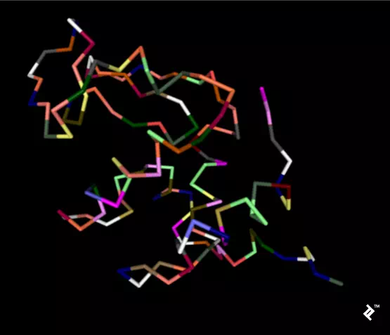
Pipes are created by joining peptide-bonded atoms with a C-alpha atom. Cysteine’s color is same as the color of sulfur in the CPK coloring method. When cystenes come close enough, their sulfurs create disulfide bonds, and that strengthens the structure. Otherwise this protein would bind too much, and its structure would be less stable at higher temperatures.

CONECT

These records are used for tagging connections between atoms. Sometimes these tags are not present at all, whereas other times all the data is filled in. In the case of analyzing disulfide bonds, this part can be useful—but it isn’t necessary. That’s because, in this project, non-tagged bonds are added by measuring distances, so this would be overhead, and also has to be checked.

SOURCE

These records contain information about the source organism from which the molecule has been extracted. They contain subrecords for easier location in taxonomy, and have the same multi-line structure we saw with title records.

SOURCE    MOL_ID: 1;                                  

SOURCE   2 ORGANISM_SCIENTIFIC: ANOPHELES GAMBIAE;    

SOURCE   3 ORGANISM_COMMON: AFRICAN MALARIA MOSQUITO; 

SOURCE   4 ORGANISM_TAXID: 7165;                      

SOURCE   5 GENE: GST1-6;                              

SOURCE   6 EXPRESSION_SYSTEM: ESCHERICHIA COLI;       

SOURCE   7 EXPRESSION_SYSTEM_TAXID: 562;              

SOURCE   8 EXPRESSION_SYSTEM_STRAIN: BL21(DE3)PLYSS;  

SOURCE   9 EXPRESSION_SYSTEM_VECTOR_TYPE: PLASMID;    

SOURCE  10 EXPRESSION_SYSTEM_PLASMID: PXAGGST1-6