Organic, Semidetached and Embedded software projects

 Boehm postulated that any software development project can be classified into one of the following three categories based on the development complexity: organic, semidetached, and embedded. In order to classify a product into the identified categories, Boehm not only considered the characteristics of the product but also those of the development team and development environment. Roughly speaking, these three product classes correspond to application, utility and system programs, respectively. Normally, data processing programs are considered to be application programs. Compilers, linkers, etc., are utility programs. Operating systems and real-time system programs, etc. are system programs. System programs interact directly with the hardware and typically involve meeting timing constraints and concurrent processing.

Organic: A development project can be considered of organic type, if the project deals with developing a well understood application program, the size of the development team is reasonably small,

Semidetached: A development project can be considered of semidetached type, if the development consists of a mixture of experienced and inexperienced staff. Team members may have limited experience on related systems but may be unfamiliar with some aspects of the system being developed.

Embedded: A development project is considered to be of embedded type, if the software being developed is strongly coupled to complex hardware, or if the stringent regulations on the operational procedures exist.

COCOMO

 COCOMO (Constructive Cost Estimation Model) was proposed by Boehm [1981]. According to Boehm, software cost estimation should be done through three stages: Basic COCOMO, Intermediate COCOMO, and Complete COCOMO.

Basic COCOMO Model

The basic COCOMO model gives an approximate estimate of the project parameters. The basic COCOMO estimation model is given by the following expressions:

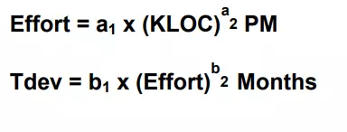
Where

•        KLOC is the estimated size of the software product expressed in Kilo Lines of Code,

•        a1, a2, b1, b2 are constants for each category of software products,

•        Tdev is the estimated time to develop the software, expressed in months,

•        Effort is the total effort required to develop the software product, expressed in person months (PMs).

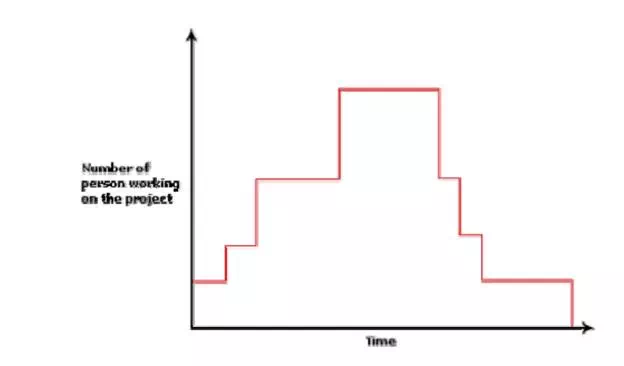
The effort estimation is expressed in units of person-months (PM). It is the area under the person-month plot . It should be carefully noted that an effort of 100 PM does not imply that 100 persons should work for 1 month nor does it imply that 1 person should be employed for 100 months, but it denotes the area under the person-month curve

Person-month curve

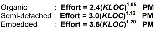
According to Boehm, every line of source text should be calculated as one LOC irrespective of the actual number of instructions on that line. Thus, if a single instruction spans several lines (say n lines), it is considered to be nLOC. The values of a1, a2, b1, b2 for different categories of products (i.e. organic, semidetached, and embedded) as given by Boehm [1981] are summarized below. He derived the above expressions by examining historical data collected from a large number of actual projects.

Estimation of development effort

For the three classes of software products, the formulas for estimating the effort based on the code size are shown below:

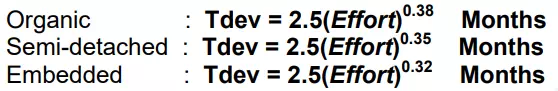
Estimation of development time

For the three classes of software products, the formulas for estimating the development time based on the effort are given below:

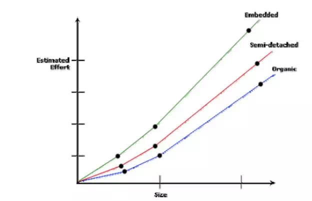
some insight into the basic COCOMO model can be obtained by plotting the estimated characteristics for different software sizes. Fig. 11.4 shows a plot of estimated effort versus product size. From fig. 11.4, we can observe that the effort is somewhat super linear in the size of the software product. Thus, the effort required to develop a product increases very rapidly with project size.

Effort versus product size

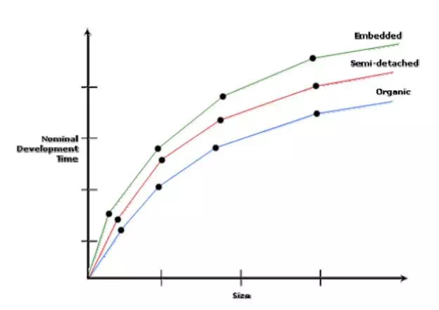
The development time versus the product size in KLOC is plotted, it can be observed that the development time is a sublinear function of the size of the product, i.e. when the size of the product increases by two times, the time to develop the product does not double but rises moderately. This can be explained by the fact that for larger products, a larger number of activities which can be carried out concurrently can be identified. The parallel activities can be carried out simultaneously by the engineers. This reduces the time to complete the project. Further, from fig. 11.5, it can be observed that the development time is roughly the same for all the three categories of products. For example, a 60 KLOC program can be developed in approximately 18 months, regardless of whether it is of organic, semidetached, or embedded type.

Development time versus size

From the effort estimation, the project cost can be obtained by multiplying the required effort by the manpower cost per month. But, implicit in this project cost computation is the assumption that the entire project cost is incurred on account of the manpower cost alone. In addition to manpower cost, a project would incur costs due to hardware and software required for the project and the company overheads for administration, office space, etc.

 It is important to note that the effort and the duration estimations obtained using the COCOMO model are called as nominal effort estimate and nominal duration estimate. The term nominal implies that if anyone tries to complete the project in a time shorter than the estimated duration, then the cost will increase drastically. But, if anyone completes the project over a longer period of time than the estimated, then there is almost no decrease in the estimated cost value.

Intermediate COCOMO model

 The basic COCOMO model assumes that effort and development time are functions of the product size alone. However, a host of other project parameters besides the product size affect the effort required to develop the product as well as the development time. Therefore, in order to obtain an accurate estimation of the effort and project duration, the effect of all relevant parameters must be taken into account. The intermediate COCOMO model recognizes this fact and refines the initial estimate obtained using the basic COCOMO expressions by using a set of 15 cost drivers (multipliers) based on various attributes of software development. For example, if modern programming practices are used, the initial estimates are scaled downward by multiplication with a cost driver having a value less than 1. If there are stringent reliability requirements on the software product, this initial estimate is scaled upward. Boehm requires the project manager to rate these 15 different parameters for a particular project on a scale of one to three. Then, depending on these ratings, he suggests appropriate cost driver values which should be multiplied with the initial estimate obtained using the basic COCOMO. In general, the cost drivers can be classified as being attributes of the following items:

Product: The characteristics of the product that are considered include the inherent complexity of the product, reliability requirements of the product, etc.

Computer: Characteristics of the computer that are considered include the execution speed required, storage space required etc.

Personnel: The attributes of development personnel that are considered include the experience level of personnel, programming capability, analysis capability, etc.

Development Environment: Development environment attributes capture the development facilities available to the developers. An important parameter that is considered is the sophistication of the automation (CASE) tools used for software development.

Complete COCOMO model

 A major shortcoming of both the basic and intermediate COCOMO models is that they consider a software product as a single homogeneous entity. However, most large systems are made up several smaller sub-systems. These subsystems may have widely different characteristics. For example, some subsystems may be considered as organic type, some semidetached, and some embedded. Not only that the inherent development complexity of the subsystems may be different, but also for some subsystems the reliability requirements may be high, for some the development team might have no previous experience of similar development, and so on. The complete COCOMO model considers these differences in characteristics of the subsystems and estimates the effort and development time as the sum of the estimates for the individual subsystems. The cost of each subsystem is estimated separately. This approach reduces the margin of error in the final estimate.

The following development project can be considered as an example application of the complete COCOMO model. A distributed Management Information System (MIS) product for an organization having offices at several places across the country can have the following sub-components:

•        Database part

•        Graphical User Interface (GUI) part

•        Communication part

Of these, the communication part can be considered as embedded software. The database part could be semi-detached software, and the GUI part organic software. The costs for these three components can be estimated separately and summed up to give the overall cost of the system.