We start this section with designing a dynamic programming algorithm for the knapsack problem: given n items of known weights w1, . . . , wn and values v1, . . . , vn and a knapsack of capacity W , find the most valuable subset of the items that fit into the knapsack. (This problem was introduced in Section 3.4, where we discussed solving it by exhaustive search.) We assume here that all the weights and the knapsack capacity are positive integers; the item values do not have to be integers.
To design a dynamic programming algorithm, we need to derive a recurrence relation that expresses a solution to an instance of the knapsack problem in terms of solutions to its smaller subinstances. Let us consider an instance defined by the first i items, 1 ≤ i ≤ n, with weights w1, . . . , wi, values v1, . . . , vi, and knapsack capacity j, 1 ≤ j ≤ W. Let F (i, j ) be the value of an optimal solution to this instance, i.e., the value of the most valuable subset of the first i items that fit into the knapsack of capacity j. We can divide all the subsets of the first i items that fit the knapsack of capacity j into two categories: those that do not include the ith item and those that do. Note the following:
Among the subsets that do not include the ith item, the value of an optimal subset is, by definition, F (i − 1, j ).
Among the subsets that do include the ith item (hence, j − wi ≥ 0), an optimal subset is made up of this item and an optimal subset of the first i − 1 items that fits into the knapsack of capacity j − wi. The value of such an optimal subset is vi + F (i − 1, j − wi).
Thus, the value of an optimal solution among all feasible subsets of the first i items is the maximum of these two values. Of course, if the ith item does not fit into the knapsack, the value of an optimal subset selected from the first i items is the same as the value of an optimal subset selected from the first i − 1 items. These observations lead to the following recurrence:

Our goal is to find F (n, W ), the maximal value of a subset of the n given items that fit into the knapsack of capacity W, and an optimal subset itself.
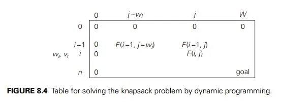
Figure 8.4 illustrates the values involved in equations (8.6) and (8.7). For i, j > 0, to compute the entry in the ith row and the j th column, F (i, j ), we compute the maximum of the entry in the previous row and the same column and the sum of vi and the entry in the previous row and wi columns to the left. The table can be filled either row by row or column by column.
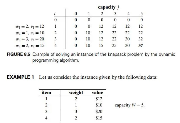
The dynamic programming table, filled by applying formulas (8.6) and (8.7), is shown in Figure 8.5.
Thus, the maximal value is F (4, 5) = $37. We can find the composition of an optimal subset by backtracing the computations of this entry in the table. Since F (4, 5) > F (3, 5), item 4 has to be included in an optimal solution along with an optimal subset for filling 5 − 2 = 3 remaining units of the knapsack capacity. The value of the latter is F (3, 3). Since F (3, 3) = F (2, 3), item 3 need not be in an optimal subset. Since F (2, 3) > F (1, 3), item 2 is a part of an optimal selection, which leaves element F (1, 3 − 1) to specify its remaining composition. Similarly, since F (1, 2) > F (0, 2), item 1 is the final part of the optimal solution {item 1, item 2, item 4}.
The time efficiency and space efficiency of this algorithm are both in (nW ). The time needed to find the composition of an optimal solution is in O(n). You are asked to prove these assertions in the exercises.
Memory Functions
As we discussed at the beginning of this chapter and illustrated in subsequent sections, dynamic programming deals with problems whose solutions satisfy a recurrence relation with overlapping subproblems. The direct top-down approach to finding a solution to such a recurrence leads to an algorithm that solves common subproblems more than once and hence is very inefficient (typically, exponential
or worse). The classic dynamic programming approach, on the other hand, works bottom up: it fills a table with solutions to all smaller subproblems, but each of them is solved only once. An unsatisfying aspect of this approach is that solutions to some of these smaller subproblems are often not necessary for getting a solution to the problem given. Since this drawback is not present in the top-down approach, it is natural to try to combine the strengths of the top-down and bottom-up approaches. The goal is to get a method that solves only subproblems that are necessary and does so only once. Such a method exists; it is based on using memory functions.
This method solves a given problem in the top-down manner but, in addition, maintains a table of the kind that would have been used by a bottom-up dynamic programming algorithm. Initially, all the table’s entries are initialized with a spe-cial “null” symbol to indicate that they have not yet been calculated. Thereafter, whenever a new value needs to be calculated, the method checks the correspond-ing entry in the table first: if this entry is not “null,” it is simply retrieved from the table; otherwise, it is computed by the recursive call whose result is then recorded in the table.
The following algorithm implements this idea for the knapsack problem. After initializing the table, the recursive function needs to be called with i = n (the number of items) and j = W (the knapsack capacity).
ALGORITHM MFKnapsack(i, j )
//Implements the memory function method for the knapsack problem //Input: A nonnegative integer i indicating the number of the first
items being considered and a nonnegative integer j indicating
the knapsack capacity
//Output: The value of an optimal feasible subset of the first i items //Note: Uses as global variables input arrays W eight s[1..n], V alues[1..n], //and table F [0..n, 0..W ] whose entries are initialized with −1’s except for //row 0 and column 0 initialized with 0’s
if F [i, j ]< 0
if j < Weights[i]
value ← MFKnapsack(i − 1, j )
else
value ← max(MFKnapsack(i − 1, j ),
Values[i]+ MFKnapsack(i − 1, j − Weights[i]))
F [i, j ] ←value return F [i, j ]
EXAMPLE 2 Let us apply the memory function method to the instance consid-ered in Example 1. The table in Figure 8.6 gives the results. Only 11 out of 20 nontrivial values (i.e., not those in row 0 or in column 0) have been computed
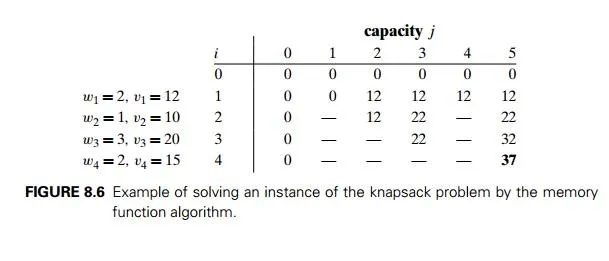
Just one nontrivial entry, V (1, 2), is retrieved rather than being recomputed. For larger instances, the proportion of such entries can be significantly larger.
In general, we cannot expect more than a constant-factor gain in using the memory function method for the knapsack problem, because its time efficiency class is the same as that of the bottom-up algorithm (why?). A more significant improvement can be expected for dynamic programming algorithms in which a computation of one value takes more than constant time. You should also keep in mind that a memory function algorithm may be less space-efficient than a space-efficient version of a bottom-up algorithm.
Exercises 8.2
a. Apply the bottom-up dynamic programming algorithm to the followinginstance of the knapsack problem:
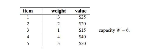
How many different optimal subsets does the instance of part (a) have?
In general, how can we use the table generated by the dynamic program-ming algorithm to tell whether there is more than one optimal subset for the knapsack problem’s instance?
a. Write pseudocode of the bottom-up dynamic programming algorithm forthe knapsack problem.
Write pseudocode of the algorithm that finds the composition of an optimal subset from the table generated by the bottom-up dynamic programming algorithm for the knapsack problem.
For the bottom-up dynamic programming algorithm for the knapsack prob-lem, prove that
its time efficiency is (nW ).
its space efficiency is (nW ).
the time needed to find the composition of an optimal subset from a filled dynamic programming table is O(n).
a. True or false: A sequence of values in a row of the dynamic programmingtable for the knapsack problem is always nondecreasing?
True or false: A sequence of values in a column of the dynamic program-ming table for the knapsack problem is always nondecreasing?
Design a dynamic programming algorithm for the version of the knapsack problem in which there are unlimited quantities of copies for each of the n item kinds given. Indicate the time efficiency of the algorithm.
Apply the memory function method to the instance of the knapsack problem given in Problem 1. Indicate the entries of the dynamic programming table that are (i) never computed by the memory function method, (ii) retrieved without a recomputation.
Prove that the efficiency class of the memory function algorithm for the knap-sack problem is the same as that of the bottom-up algorithm (see Problem 3).
Explain why the memory function approach is unattractive for the problem of computing a binomial coefficient by the formula C(n, k) = C(n − 1, k − 1) +
C(n −1, k).
Write a research report on one of the following well-known applications of dynamic programming:
finding the longest common subsequence in two sequences
optimal string editing
minimal triangulation of a polygon

Comments are closed