
A ticket sale opens at noon. Within seconds, thousands of people refresh the same page, add seats to their carts, and attempt to pay. The application may have plenty of servers available, yet users can still see timeouts if too many requests land on one machine.
The same pattern appears in food-delivery apps during dinner, learning platforms before an exam deadline, and internal systems on payroll day. Traffic is not only large; it is uneven, unpredictable, and made of requests with very different costs.
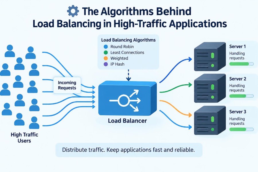
A load balancer sits at a critical junction. It decides where incoming work should go, usually before the application code handles it. That decision can be simple, such as rotating through a list of servers, or adaptive, using live signals about latency, connections, and capacity.
Understanding the algorithms behind that choice helps engineers design systems that stay responsive under pressure, diagnose strange performance problems, and avoid treating “more servers” as a complete scaling strategy.
🚦 What Load Balancing Actually Does
Load balancing distributes incoming work across multiple resources: application instances, database replicas, queues, network paths, or geographic regions. Most discussions focus on a reverse proxy or dedicated service receiving client requests and selecting an upstream server.
Its goal is not merely equal request counts. A useful balance keeps response times acceptable, avoids overloaded components, uses available capacity efficiently, and continues serving traffic when individual instances fail.
“Work” can mean an HTTP request, a persistent WebSocket connection, a TCP flow, a background job, or a query. The right algorithm depends on which kind of work is being assigned.
🏢 Why Equal Requests Are Not Equal Work
Imagine two API requests. One reads a small cached profile; another generates a report that performs several database queries and returns a large file. Counting both as one request hides a major difference in CPU time, memory use, network output, and connection duration.
This is why a perfectly even request distribution can still create uneven server load. Load balancers make decisions with incomplete information, so their measurements are proxies for real cost rather than direct measures of every operation.
Applications with fairly uniform, short requests can use simple policies successfully. Systems with variable processing times often need adaptive policies, explicit capacity weights, queues, or application-level workload controls.
🧭 The Request Path and Decision Points
A client commonly resolves a domain name, connects to an edge or regional load balancer, completes transport security negotiation, and sends a request. The balancer checks which targets are eligible, applies a routing policy, and forwards the request.
Decisions can happen at several layers. A DNS service may choose a region, a layer 4 balancer may choose a TCP target, and a layer 7 proxy may route a particular HTTP path to a specialized service.
Each layer sees different information. Lower layers are fast and protocol-agnostic; higher layers can inspect hostnames, paths, headers, and sometimes cookies, but usually consume more processing resources.
🔄 Round Robin: The Baseline Algorithm
Round robin cycles through healthy servers in order: A, then B, then C, then back to A. It is easy to understand, predictable, and often adequate when instances have similar capacity and requests have similar duration.
Its weakness is that it assumes the next server is as available as the others. If server B is handling several expensive requests, round robin still sends it its scheduled share. It also does not inherently account for a slower machine, a noisy neighbor in a virtualized environment, or a warming cache.
Round robin remains valuable as a baseline because it is simple to test. If a more complex algorithm performs worse, the extra signals or assumptions deserve scrutiny.
⚖️ Weighted Round Robin for Unequal Capacity
Weighted round robin gives stronger targets more turns. In a hypothetical pool with weights of 4, 2, and 1, the first server should receive roughly four times as many selections as the third over a sufficiently large number of requests.
Weights are useful during gradual hardware upgrades, mixed instance types, or controlled canary deployments. They can also reduce traffic to a service that is intentionally operating with reduced capacity.
Static weights have limits. They describe expected capacity, not current health. A high-weight server suffering a dependency slowdown can still receive too much traffic until health checks or dynamic controls intervene.
👥 Least Connections and Long-Lived Sessions
Least connections sends a new connection to the eligible server with the fewest active connections. This is often a better fit than round robin for WebSockets, streaming responses, or other workloads where connections remain open for very different lengths of time.
Connection count is still an imperfect measure. Ten idle WebSockets may cost less than one active request performing intensive computation. Conversely, a server with few connections may be saturated by CPU-heavy work.
Many implementations combine the idea with weights, comparing active connections relative to a target’s capacity. This prevents a smaller server from being treated as equivalent to a much larger one.
⏱️ Least Response Time and Feedback Signals
A response-time-aware policy favors targets that have recently answered quickly. It treats latency as feedback: if a server becomes slower, new requests shift elsewhere before it necessarily fails a health check.
This can improve user-facing performance, but the signal is noisy. A slow response may come from the network, a downstream database, a particular endpoint, or an unusually expensive request. Moving all traffic away too quickly can make another server the next bottleneck.
Well-designed adaptive systems smooth measurements over time and avoid reacting to one outlier. They also need safeguards so an apparently fast but under-tested target is not flooded instantly.
🎲 Random Selection and the Power of Two Choices
Choosing a healthy server at random sounds unsophisticated, but it distributes traffic surprisingly well in large pools and avoids the shared counter required by strict round robin. Randomness can reduce synchronization hotspots in distributed balancer implementations.
A widely useful variation is power of two choices: select two eligible targets randomly, compare their current load, and send work to the better one. “Better” might mean fewer active requests, fewer connections, or lower estimated latency.
This gains much of the benefit of global least-load selection without inspecting every server on every decision. It is especially practical when a very large fleet makes exact global state costly or stale.
🧮 How Algorithms Estimate Load
No single metric captures load for every application. A balancer may observe active connections, in-flight requests, response time, error rate, CPU utilization, queue depth, or an application-reported capacity score.
| Signal | Useful when | Blind spot |
|---|---|---|
| Active connections | Sessions persist for varying lengths | Connection cost varies widely |
| In-flight requests | Request duration reflects pressure | May miss CPU saturation after requests finish |
| Recent latency | User response time is the priority | Can reflect downstream issues |
| CPU or queue depth | Targets report reliable local state | Metrics can arrive late or be unavailable |
The key question is practical: which signal changes early enough to prevent overload and closely enough reflects the resource your application actually exhausts?
🩺 Health Checks Determine Who Can Receive Traffic
Before choosing among targets, a balancer needs an eligible set. Health checks periodically test whether a target should receive new work, often through a TCP connection, an HTTP endpoint, or an application-specific probe.
A basic check answers, “Is the process reachable?” A deeper check might verify that the application can serve a lightweight request. Checking every dependency in that endpoint can be dangerous: a temporary database problem could remove every application instance at once, even when some requests could still succeed.
Health checks should match the traffic decision they control. They are not a substitute for observability or full end-to-end monitoring.
🧯 Failure Detection Is a Trade-Off
Fast failure detection limits the number of requests sent to a broken target. But aggressive thresholds can mistake a short network disturbance for a real outage and repeatedly remove and restore healthy instances.
This oscillation is often called flapping. It can amplify instability because returning traffic changes the very conditions being measured.
Useful controls include consecutive-success and consecutive-failure thresholds, timeouts, a slow-start period after recovery, and separate handling for connection failures versus ordinary application errors. The correct values depend on traffic patterns and recovery behavior, not a universal template.
🐢 Slow Start Prevents Recovery From Becoming Overload
A newly started or recovered server may be technically healthy but practically unready. Its caches are cold, connection pools are empty, just-in-time compilation may still occur, and it may need to load data or establish secure connections.
Slow start gradually increases the fraction of new traffic sent to that server. Rather than returning it immediately to full weight, the balancer ramps capacity over a configured interval or as performance remains stable.
This mechanism is particularly helpful after autoscaling events and rolling deployments. It does not fix slow startup itself, but it gives the instance room to become useful without turning recovery into another incident.
🍪 Session Persistence and the Cost of Stickiness
Some applications need a user to return to the same server, commonly called session persistence or sticky sessions. A balancer can use a cookie, source address, or connection affinity to preserve that mapping.
Stickiness simplifies applications that store session state in process memory. It also weakens balancing: a popular user, a long-lived session, or an uneven client network can pin disproportionate work to one target.
Where feasible, externalizing session state to a shared store or using signed stateless tokens lets requests move freely. That introduces its own design and security considerations, but it usually improves resilience during instance replacement.
🧩 Consistent Hashing for Stable Placement
Consistent hashing maps a key, such as a cache key or tenant ID, to a position on a conceptual ring and assigns nearby positions to servers. When servers are added or removed, only a portion of keys need to move.
This differs from simple modulo hashing, where changing the number of servers can remap a large share of keys. Stable placement is useful for distributed caches, sharded services, and workloads where local data reuse matters.
Real implementations usually use multiple virtual positions per server to improve distribution. Even then, hot keys remain possible: if one tenant or object becomes extremely popular, hashing faithfully routes its traffic to the same place.
🗺️ Geographic Routing Is Another Balancing Layer
High-traffic systems often balance across regions before balancing across individual instances. Geographic routing may favor a nearby region to reduce network delay, or route based on regional capacity and service availability.
“Nearest” is not always best. Internet routes are complex, a nearby region may be under stress, and data residency or replication rules can limit where a request is allowed to go.
Multi-region architectures also make state harder. Sending a user to another region is only safe when authentication, data access, and writes are designed for that possibility. Routing policy cannot compensate for inconsistent data design.
🌐 DNS Balancing and Its Caching Limits
DNS can distribute clients among addresses or regions before a connection begins. It is inexpensive and broadly compatible, but it offers limited control after an answer is cached by clients, operating systems, resolvers, and intermediate networks.
A short DNS time-to-live can encourage quicker changes, but it does not guarantee every client will switch exactly on schedule. DNS also cannot see individual request latency or connection counts at the application tier.
For these reasons, DNS commonly provides coarse regional steering, while a local load balancer performs fine-grained balancing among instances.
📦 Layer 4 and Layer 7 Make Different Choices
A layer 4 balancer routes using transport-level information such as IP addresses and TCP or UDP ports. It can be efficient and protocol-neutral, which is useful for non-HTTP traffic.
A layer 7 balancer understands application protocols such as HTTP. It can route /images to one service, /api to another, apply request-aware rules, and make decisions based on headers or methods.
Layer 7 flexibility comes with more responsibility: request parsing, security configuration, connection management, and protocol-specific failure behavior. The better layer is the one that exposes the information needed without creating unnecessary complexity.
🧵 Connection Reuse Changes the Distribution
Modern clients and proxies reuse connections through keep-alive, HTTP/2, and HTTP/3. That is efficient, but it means a balancing decision may occur once per connection rather than once per request.
If one client connection carries many requests, connection-level balancing can produce skew. HTTP/2 adds multiplexing, where several concurrent streams share one connection, making “active connection count” even less representative of active work.
Architectures can address this by terminating connections at a proxy that distributes requests upstream, or by choosing metrics suited to long-lived, multiplexed connections. The correct approach depends on protocol support and latency requirements.
🚧 Queues, Backpressure, and Admission Control
A load balancer cannot create capacity. When all targets are saturated, blindly forwarding more work increases queueing delay until requests time out, clients retry, and pressure grows further.
Backpressure means signaling that the system cannot safely accept more work. It may involve bounded queues, rate limits, returning an explicit overload response, or prioritizing critical traffic over optional operations.
For asynchronous jobs, a queue smooths bursts by separating acceptance from processing. For synchronous user requests, queues must remain short and bounded; a long queue often turns a fast rejection into a slow, resource-consuming failure.
🔁 Retries Can Multiply an Outage
A retry is reasonable when a request fails due to a brief, isolated problem. During broad overload, automatic retries may send the same operation repeatedly to an already struggling fleet.
Safe retry design uses deadlines, limited attempts, exponential backoff, and random jitter so clients do not retry in synchronized waves. Requests that change data also need idempotency protection, meaning repeated delivery does not accidentally create duplicate actions.
Load balancing and retries must be designed together. A balancer may select a healthy destination, but retry traffic can still consume the capacity needed for first attempts.
📈 Autoscaling Is Related but Not the Same
Load balancing decides where current work goes. Autoscaling decides whether the system should have more or fewer resources. They operate on different time scales: routing can change in milliseconds, while launching and warming new instances can take much longer.
A common failure mode is treating autoscaling as an instant escape hatch. If demand rises faster than new capacity becomes ready, the existing fleet must survive the gap through headroom, queueing policies, caching, and admission control.
Scaling signals should also reflect the bottleneck. CPU may be useful for compute-bound services, while queue depth, concurrency, or latency can be more meaningful for I/O-bound workloads.
🧊 Caching Reduces Work Before Balancing Begins
The cheapest request to balance is often the one that never reaches the application fleet. Browser caches, content delivery networks, reverse-proxy caches, and application caches can absorb repeat reads and static assets.
Caching is not just a performance optimization; it changes the workload shape the balancer sees. A cache miss can be much more expensive than a hit, so sudden expiry of many entries can create a burst against origin servers.
Engineers should plan for cache stampedes with request coalescing, staggered expiry, stale-while-revalidate patterns where appropriate, and capacity for a miss-heavy period.
🔍 Observability Shows Whether “Balanced” Means Healthy
Dashboards that show only total requests are insufficient. A balanced system can have equal traffic per instance while one target has worse latency, more errors, or a growing queue.
Track distributions, not only averages. Useful views include per-target request rate, concurrency, latency percentiles, error classes, saturation signals, health-state transitions, and the number of requests rejected or queued.
Correlate balancer logs with application traces when possible. A slow request may reveal whether the delay occurred before routing, while waiting for a connection, inside an application handler, or in a downstream dependency.
🧪 Test the Failure Modes, Not Only the Happy Path
A load test that sends identical requests to healthy servers verifies only a narrow slice of behavior. More revealing tests introduce uneven request costs, slow targets, dropped connections, dependency latency, a draining instance, and a sudden traffic spike.
In a safe test environment, deliberately make one target slower and observe whether routing shifts gradually, whether health checks flap, and whether retries create extra load. Test persistent connections separately from short requests.
Chaos-style experiments should be controlled and reversible. Their purpose is not disruption; it is to validate assumptions before an unplanned event does so under real customer traffic.
🛠️ Choosing an Algorithm by Workload
There is no universal winner. Start with the shape of work, the accuracy and cost of available metrics, and the operational failure modes you can observe.
- Use round robin for similar, short-lived requests on comparable instances.
- Use weighted routing when capacity intentionally differs among targets.
- Use least connections when session duration dominates variation.
- Use latency-aware or least-request policies when live service pressure varies substantially.
- Use consistent hashing when stable key placement improves cache locality or shard ownership.
Then validate the choice under realistic traffic. An algorithm is only as good as its assumptions about workload and target behavior.
⚠️ Common Design Mistakes
One mistake is using a single global metric as if it explains every bottleneck. Another is creating sticky sessions by default, then discovering that safe instance replacement and even distribution have become difficult.
Other recurring problems include unbounded queues, health checks that overload dependencies, retry policies without jitter, and dashboards that hide per-instance outliers behind fleet averages.
Perhaps the most subtle mistake is assuming a balancer can solve downstream contention. If every request waits on the same database lock or third-party API, redistributing requests only spreads the waiting across more application servers.
🧱 A Practical Design Checklist
Before selecting or tuning a policy, write down the decisions your system must make and the evidence it can trust.
- Classify traffic: short HTTP calls, streams, WebSockets, jobs, or a mixture.
- Identify the limiting resources: CPU, memory, database connections, bandwidth, or a dependency quota.
- Define health separately from capacity and decide what each check should prove.
- Choose bounded overload behavior: reject, queue, shed optional work, or defer it.
- Measure per-target outcomes and rehearse target removal, recovery, and rapid growth.
This process often reveals that a routing algorithm is only one part of a broader capacity and resilience design.
🎯 The Core Principle: Route With Context, Design for Limits
Load balancing is a feedback problem. The balancer makes a decision using a model of target availability, then observes outcomes through latency, errors, connection counts, or application signals. Better algorithms improve that model, but none removes uncertainty.
The strongest designs combine a sensible routing policy with health checks, gradual recovery, observability, caching, bounded queues, careful retries, and enough capacity margin for the time autoscaling needs to react.
Simple policies are often the right starting point because they are explainable. Add sophistication when you can name the workload behavior it addresses and measure whether the added complexity improves real outcomes.
The best load-balancing algorithm is the one whose assumptions match your workload, whose failures are contained, and whose behavior your team can observe and operate. Build for uneven work and imperfect signals, and high traffic becomes a manageable engineering problem rather than a guessing game. ⚙️📈🛡️