This is a list of non-redundant (NR) chain PDB sets. Its snapshots can be found at ftp.ncbi.nih.gov/mmdb/nrtable/. Its purpose is to avoid unnecessary biases caused by protein similarity. NR has three sets with different identity p-value levels created by comparison of all PDB structures. The result is added to textual files which will be explained later. Not all columns are needed for this project, so only the important ones will be explained.
The first two columns contain the unique PDB experiment code and the chain identifier as explained for ATOM records above. Columns 6, 9, and C contain information about p-value representativity, which is the level of similarity of sequences calculated by BLAST. If that value is zero, then it is not accepted to be part of a set; if the value is 1, then it is. The mentioned columns represent the acceptance of sets with p-values cutoffs of 10e-7, 10e-40, and 10e-80, respectively. Only sets with a p-value cutoff of 10e-7 will be used for analysis.
The last column contains info about a structure’s acceptability, where a is acceptable and n is not.
#---------------------------------------------------------------------------------------------------------------------------# 1 2 3 4 5 6 7 8 9 A B C D E F G H I J K L M N O P Q#---------------------------------------------------------------------------------------------------------------------------3F8V A 69715 1 1 1 1 1 1 1 1 1 9427 1 1 0.00 0.00 0.00 0.00 1.08 1 6 5 164 X a3DKE X 68132 1 2 0 1 2 0 1 2 0 39139 1 1 0.00 0.00 0.00 0.00 1.25 1 11 7 164 X a3HH3 A 77317 1 3 0 1 3 0 1 3 0 90 1 0 0.00 0.00 0.00 0.00 1.25 1 5 4 164 X a3HH5 A 77319 1 4 0 1 4 0 1 4 0 90 2 0 0.00 0.00 0.00 0.00 1.25 1 4 4 164 X aDatabase Construction and Parsing Data
Now that we have an idea of what we’re dealing with and what we need to do, let’s get started.
Parsing Data
Usually the parsing of PDB files is done by plugins or modules in Java, Perl, or Python. In the case of this research, I wrote a custom Perl application without using a pre-written PDB-parsing module. The reason for that is when parsing a large quantity of data, in my experience, the most common problem with using experimental data is errors in the data. Sometimes there are errors with coordinates, distances, line lengths, comments in places where they shouldn’t be, etc.
The most effective way to deal with this is to initially store everything in the database as raw text. Common parsers are written to deal with ideal data that conforms completely to specifications. But in practice, data is not ideal, and that will be explained in filtering section where you’ll find the Perl import script.
Database Construction
When constructing the database, note that this database is built for processing data. Later analysis will be done in SPSS or R. For our purposes here it is recommended to use PostgreSQL with at least version 8.4.
The table structure is directly copied from the downloaded files with only a few small changes. In this case, the number of records is far too small for it to be worth spending our time on normalization. As mentioned, this database is single-use only: These tables aren’t built to be served on a website—they are just there for processing data. Once that is finished, they can be dropped, or backed up as supplementary data, perhaps for repeating the process by some other researcher.
In this case, the final result will be one table which can then be exported to a file for use with some statistical tool like SPSS or R.
Tables
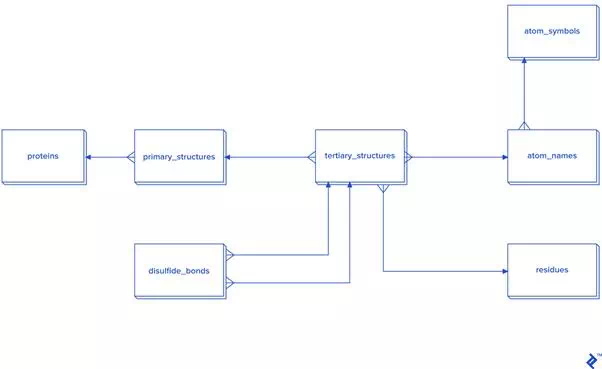
Data extraction from ATOM records has to be connected to HEADERor TITLE records. The data hierarchy is explained in the picture below.

Since this picture is a simplified representation of a database in the third normal form (3NF), for our purposes it contains too much overhead. The reason: To calculate the distance between atoms for disulfide bond detection, we would need to do joins. In this case, we would have a table joined to itself twice, and also joined to a secondary and primary structure twice each, which is a very slow process. Since not every analysis needs secondary structure information, another schema is proposed in case you need to reuse data or analyze bigger quantities of disulfide bonds:

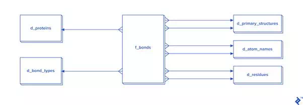
Disulfide bonds are not so frequent as other covalent bonds are, so a warehouse model is not needed, although it could be used. The star schema and dimensional modeling below will take too much time to develop, and will make queries more complex:

In cases where all bonds have to be processed, then I recommend the star schema.
(Otherwise it’s not needed, because disulfide bonds aren’t as common as other bonds are. In the case of this work, the number of disulfide bonds is near 30,000, which may be fast enough in 3NF, but I decided to process it via a non-normalized table, so it isn’t pictured here.)
The expected total number of all covalent bonds is at least twice the number of atoms in the tertiary structure, and in that case 3NF would be very slow, so denormalization using the star schema form is needed. In that schema, some tables have two foreign key checks, and that is because a bond is created between two atoms, so each atom needs to have its own primary_structure_id, atom_name_id and residue_id.
There are two ways to fill the d_atom_name dimension table: from data, and from another source, the chemical component dictionary I mentioned earlier. Its format is similar to the PDB format: Only RESIDUE and CONECT lines are useful. This is because RESIDUE’s first column contains a residue three-letter code, and CONECTcontains the name of the atom and its connections, which are also atom names. So from this file, we can parse all atom names and include them in our database, although I recommend you allow for the possibility of the database containing unlisted atom names.
RESIDUE PRO 17CONECT N 3 CA CD H CONECT CA 4 N C CB HA CONECT C 3 CA O OXT CONECT O 1 C CONECT CB 4 CA CG HB2 HB3 CONECT CG 4 CB CD HG2 HG3 CONECT CD 4 N CG HD2 HD3 CONECT OXT 2 C HXT CONECT H 1 N CONECT HA 1 CA CONECT HB2 1 CB CONECT HB3 1 CB CONECT HG2 1 CG CONECT HG3 1 CG CONECT HD2 1 CD CONECT HD3 1 CD CONECT HXT 1 OXT END HET PRO 17HETNAM PRO PROLINEFORMUL PRO C5 H9 N1 O2In this project, speed of coding is more relevant than speed of execution and storage consumption. I decided not to normalize—after all, our goal is to generate a table with the columns mentioned in the intro.
In this part, only the most important tables will be explained.
The main tables are:
· proteins: Table with experiment names and codes.
· ps: Primary structure table which will contain sequence, chain_id, and code.
· ts: Table containing tertiary/quaternary structure extracted from raw data and transformed into ATOM record format. This will be used as a staging table, and can be dropped after extraction. Ligands are excluded.
· sources: The list of organisms from which experimental data was derived.
· tax_names, taxonomy_path, taxonomy_paths: Linnean taxonomy names from the NCBI taxonomy database, used to get taxonomy paths from organisms listed in sources.
· nr: List of NCBI non-redundant proteins extracted from the NR set.
· pdb_ssbond: List of disulfide bonds in a given PDB file.

