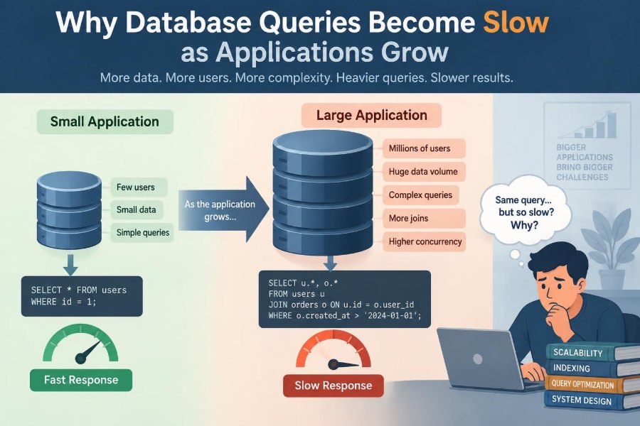

A product can feel fast for months, even years. A customer searches for an order, opens a dashboard, or loads a message thread, and the result appears almost immediately.
Then the application grows. More customers arrive, old records accumulate, teams add reporting screens, and a feature that once queried a few hundred rows quietly begins touching millions. The database has not suddenly become “bad”; the workload has changed.
This is a familiar and expensive engineering problem because slow queries affect more than a single screen. They consume shared resources, hold up other requests, exhaust connection pools, and can turn a small spike in traffic into a wider outage.
Understanding why queries slow down helps teams make better design choices early, diagnose production problems calmly, and improve performance without guessing.
🧭 A query is a request for work
A database query is not merely a line of SQL. It is an instruction to find, combine, sort, calculate, and return data. The apparent simplicity of SELECT * FROM orders WHERE customer_id = 42 hides several decisions about where data lives and how it should be read.
For a small table, many reasonable strategies are fast enough. As data and traffic grow, the cost of each strategy becomes visible. Query performance is therefore about the amount of work required to produce a result, not just the syntax of the statement.
📈 Growth changes several dimensions at once
Applications rarely grow in only one way. Row counts rise, but so do simultaneous users, the number of related tables, the size of individual records, and expectations for real-time reporting.
A query that reads 1% of a table may be harmless when that table has 10,000 rows. At 100 million rows, that same percentage is a million rows to inspect. Meanwhile, more concurrent requests may compete for the same CPU, memory, disk, and network capacity.
🔎 Full table scans become costly
A full table scan means the database reads every row in a table, testing whether each row matches the query condition. This can be appropriate for small tables or for reports that genuinely need most rows.
It becomes troublesome when an interactive request needs only a few records but lacks an efficient way to locate them. For example, searching users by email without an appropriate index can require examining the entire users table as it grows.
A scan is not automatically a bug. The key question is whether reading the whole table is proportionate to the result needed.
🗂️ Indexes provide a faster path
An index is a data structure that helps a database locate rows without reading every row first. It is similar to a book index: rather than turning every page to find a topic, you use a maintained lookup structure that points toward relevant pages.
Indexes often help filters, joins, ordering, and uniqueness checks. But they are not magical speed switches. They consume storage, must be maintained whenever data changes, and only help when their structure matches the query’s access pattern.
🧩 The wrong index is almost like no index
Suppose an order screen frequently asks for a customer’s newest orders:
SELECT id, total, created_at
FROM orders
WHERE customer_id = ?
ORDER BY created_at DESC
LIMIT 20;
An index on customer_id may reduce the search space, but the database might still need to sort all of that customer’s matching orders. A composite index that begins with customer_id and includes created_at may better match the filter and ordering.
Index design depends on the actual predicates, sort order, join keys, and database engine. Copying indexes from a generic checklist often creates write overhead without solving the slow query.
🧱 Composite index column order matters
A composite index stores values in a particular column sequence. An index on (status, created_at) is organized differently from one on (created_at, status), even though both mention the same columns.
Typically, equality conditions are useful early in the index path, followed by columns used for ranges or ordering. But selectivity matters too: a column with only a few values, such as a boolean flag, may not narrow the search much by itself.
Use the query plan and representative data to validate the order. Database optimizers have engine-specific behavior, so rules of thumb should start an investigation, not end one.
🔗 Joins multiply the work
Joins connect rows across tables, such as orders to customers and order items. They are fundamental to relational databases, but their cost depends on how many rows enter each stage and how the database finds matching rows.
A join that starts with a narrowly filtered set can be efficient. A join that combines two large, weakly filtered sets can create enormous intermediate results before the final conditions remove most of them.
Indexes on join columns are often essential, especially on the side of a relationship that is repeatedly searched for matches.
🪢 Many-to-many relationships need extra care
Tables that model memberships, tags, permissions, or product categories often sit between two entities. A user may belong to many groups, and each group may contain many users.
These bridge tables can grow surprisingly quickly. A query that joins users, memberships, groups, and permissions may duplicate rows at several stages before aggregation removes duplicates. The result may be correct but unnecessarily expensive.
Keep the join path intentional, index both foreign-key directions where workloads need them, and avoid joining broad relationship tables before applying selective filters.
🔁 The N+1 query pattern adds round trips
The N+1 problem occurs when code loads a list with one query, then sends another query for each item in that list. A page showing 50 projects may run one query for projects plus 50 queries for project owners.
Each small query may look fast in isolation. Together, they add network round trips, parsing work, connection usage, and load on shared database resources. Under concurrency, the effect is much worse.
Batch loading, carefully chosen joins, or application-level preloading can reduce this pattern. The right option depends on the data shape; one huge join is not always safer than several bounded queries.
📦 Fetching too much data wastes resources
SELECT * is convenient during exploration, but production code often needs fewer columns than it requests. Wide text fields, JSON documents, binary values, or rarely used metadata increase disk reads, memory use, serialization time, and network transfer.
Returning 1,000 rows when a screen displays 20 creates a similar problem. The database does work, the application allocates memory, and the network carries data that nobody uses.
Select only required columns and use explicit, stable pagination for lists. This is both a performance improvement and a clearer statement of the interface the query serves.
📄 Offset pagination gets slower deeper in a list
Offset pagination commonly looks like LIMIT 20 OFFSET 100000. Although it returns only 20 rows, the database may still need to find, order, and skip a large number of earlier rows.
For long, ordered lists, keyset pagination is often more scalable. Instead of asking to skip 100,000 rows, the client asks for rows after a known boundary, such as a timestamp and unique identifier from the previous page.
Keyset pagination requires a deterministic sort order and careful handling of ties. It is not always suitable for arbitrary page jumps, but it is often a better match for feeds and sequential browsing.
↕️ Sorting can spill beyond memory
An ORDER BY clause may require the database to sort many candidate rows. If no useful index provides the desired order, sorting uses memory and may temporarily write data to disk when the working set is too large.
Sorting becomes especially expensive after broad joins or when a query sorts before applying a restrictive limit. A dashboard that asks for “the newest 20 events” should not need to sort an entire event history if an appropriate access path exists.
Query plans can reveal explicit sort operations and whether they are processing far more rows than the final result.
🧮 Aggregations grow with the input set
Counts, sums, averages, distinct values, and grouped reports are valuable, but they must inspect and combine data. A daily revenue report over recent orders differs greatly from a request that calculates several years of metrics during every page load.
COUNT(*) is not universally cheap. Its cost depends on the database system, visibility rules, filters, indexes, and number of rows involved. Treating it as free can create unpleasant surprises on large transactional tables.
For frequently requested summaries, consider pre-aggregated tables, materialized views where supported, or carefully designed asynchronous reporting pipelines.
🧷 DISTINCT can hide a modeling or join problem
Developers sometimes add DISTINCT to remove duplicate results from a join. It may fix the visible output, but it asks the database to identify and eliminate repeated rows, often through sorting or hashing.
The duplicates may be legitimate consequences of a one-to-many relationship. If the page needs one row per customer, joining every order and then deduplicating customers may be the wrong shape of query.
Sometimes EXISTS, a subquery, or aggregation expresses the intention more directly. Inspect why duplicates appeared before treating DISTINCT as a default remedy.
🧠 Functions can prevent efficient searching
Conditions that transform a column can make an ordinary index difficult to use. For example, filtering with WHERE DATE(created_at) = ... may require applying a function to many stored values before comparison.
A range condition is often friendlier to indexing: compare created_at against the start and end of the desired period. The exact syntax and time-zone handling must match the application’s requirements.
Other examples include leading wildcard searches such as LIKE '%term', implicit type conversions, and expressions on join keys. Some databases offer functional indexes or specialized search indexes, but these should reflect a measured need.
🗺️ The optimizer chooses a plan from estimates
Most relational databases use a query optimizer. It evaluates possible execution plans—different join orders, indexes, and algorithms—and chooses one based on estimated cost.
Its estimates depend on statistics about data distribution. If values are skewed, statistics are stale, or predicates are complex, the optimizer can misjudge how many rows a step will return and choose a poor plan.
This explains why a query can be fast for one parameter and slow for another. A query for a rare status may behave very differently from one for a status held by most rows.
🔬 Execution plans replace guesswork
An execution plan describes the work the database intends to perform. Many systems provide an EXPLAIN command, and some can show actual row counts and timing when configured appropriately.
Look for discrepancies between estimated and actual rows, unexpected full scans, expensive sorts, repeated nested operations, and large intermediate results. The exact terminology differs by database, but the diagnostic question stays the same: where is the query doing more work than expected?
Plans should be read alongside the query, schema, indexes, and realistic parameter values. A plan alone does not prove that an index is needed.
🧪 Test plans with realistic data distributions
A local database with a few thousand evenly distributed records rarely reveals production behavior. Real systems have old accounts with unusually large histories, popular products, deleted-but-retained records, and values that cluster around certain dates or statuses.
Create safe representative datasets when possible, including skew and large parent-child relationships. Test the parameters that represent common traffic as well as known “heavy” cases.
Performance testing does not need perfect production duplication to be useful. It needs enough realism to expose changes in query shape and resource use.
🔒 Locks and long transactions create waiting
A slow request is not always spending time reading data. It may be waiting for another transaction to release a lock or finish work that affects the same rows or structures.
Long transactions can hold locks longer than intended, delay cleanup of old row versions, and increase contention. A transaction that performs user interaction, external API calls, or large batches before committing is particularly risky.
Keep transactions focused and short. Choose isolation levels deliberately, because stronger isolation can provide important correctness guarantees while increasing coordination costs for certain workloads.
🧹 Updates make indexes more expensive
Every additional index improves some reads at a price. When a row is inserted, updated, or deleted, the database may also need to update each relevant index.
On a write-heavy table, adding many speculative indexes can slow ingestion, increase storage, and complicate maintenance. Indexes should support observed, high-value query patterns rather than every column that seems searchable.
The balanced goal is not “maximum indexes.” It is an index set that supports critical reads while preserving acceptable write performance.
🧱 Table and index bloat affect physical work
Some database engines retain old row versions or leave space behind after updates and deletes until maintenance processes reclaim or reorganize it. Over time, tables and indexes can become physically larger than their live data suggests.
Larger structures mean more pages to read and less effective cache use. Maintenance settings, vacuuming or cleanup behavior, update patterns, and long-running transactions can all influence this outcome.
This is engine-specific operational territory. Measure before acting, and follow the database vendor’s guidance for maintenance rather than applying destructive fixes casually.
💾 Memory caches help until the working set outgrows them
Databases cache frequently used data pages in memory. When a query reads data already in cache, it can avoid slower storage access. When its working set is larger than available memory, more reads must come from storage.
Growth can therefore produce a gradual performance decline even without a code change. A larger table, more competing queries, or a new report may displace pages that the main application previously reused effectively.
More memory can help, but it cannot repair a query that unnecessarily reads vast amounts of data. Reduce avoidable work before assuming hardware is the answer.
🌐 Network and application overhead still count
Database latency includes more than execution time. A request may wait for a connection, travel across a network, serialize a large result set, and be processed by application code before a user sees it.
Connection pools are designed to limit concurrent database connections. If queries hold connections too long, requests queue at the pool even when the database itself appears only moderately busy.
Measure end-to-end timing alongside database timing. This separates a slow SQL operation from an application that issues too many queries or transfers too much data.
🚦 Concurrency turns minor inefficiency into pressure
A query that takes 100 milliseconds may seem acceptable in isolation. If many requests run it simultaneously, each holding memory, CPU, locks, or a connection, the shared cost can become substantial.
Queueing makes this nonlinear in practice. As utilization approaches a resource limit, waiting grows, which increases the number of in-flight requests and can create a feedback loop.
That is why performance work should consider throughput and concurrency, not only the duration of a single hand-picked request.
📊 Reporting workloads compete with transactional work
Transactional queries support actions such as placing an order or updating a profile. Analytical queries scan, group, and compare larger periods of data. Running both against the same primary database can be reasonable at small scale, but their needs differ.
| Workload | Typical pattern | Primary concern |
|---|---|---|
| Transactional | Small reads and writes by key | Low latency and correctness |
| Analytical | Large scans, grouping, historical comparisons | Throughput across many rows |
Read replicas, warehouses, materialized summaries, or separate reporting stores can reduce interference. These designs introduce freshness and operational trade-offs, so they should solve a demonstrated workload conflict.
🧊 Caching is useful but changes consistency
Caching a popular result can reduce repeated database work, especially for data that changes infrequently. It can exist in application memory, a shared cache, a content layer, or as precomputed database results.
The difficult question is invalidation: when the underlying data changes, when should the cache be refreshed or removed? Stale data may be acceptable for a public popularity list and unacceptable for an account balance.
Use caching after understanding the query and its correctness needs. A cache can protect a database, but it can also conceal inefficient access patterns until a cache miss occurs.
🪓 Partitioning changes where data is searched
Partitioning divides a large logical table into smaller physical pieces, often by time, tenant, or another boundary. A query that includes the partition key may allow the database to ignore irrelevant partitions, a process often called partition pruning.
It is especially useful when access naturally follows the chosen boundary, such as recent events by date. Queries that omit that boundary may still touch many partitions and gain little.
Partitioning adds operational complexity: constraints, indexes, retention rules, migrations, and uneven data distribution all require planning. It is not a substitute for sound query design.
🧭 Sharding solves a different scaling problem
Sharding distributes data across multiple database instances. It can increase total capacity by assigning different tenants or key ranges to different shards.
However, cross-shard joins, global uniqueness, reporting, rebalancing, and operational recovery become more difficult. A poorly indexed query remains poorly indexed after sharding; it merely runs against a smaller slice of data.
Consider sharding when a clear distribution key and sustained capacity need justify the complexity, not as an early reaction to one slow endpoint.
🛠️ A disciplined tuning workflow
Reliable performance work follows evidence. Start with the user-facing symptom and identify the exact query or query pattern responsible. Then compare its behavior under representative inputs.
- Measure latency, call frequency, rows returned, and rows examined where available.
- Capture the query shape and relevant parameter categories without exposing sensitive values.
- Inspect the execution plan and schema indexes.
- Form one hypothesis, such as a missing composite index or broad join.
- Change one thing, test correctness and write impact, then measure again.
- Monitor after deployment because live distributions and concurrency can differ from tests.
This workflow prevents the common habit of adding indexes or infrastructure changes without knowing which cost they address.
⚠️ Common “fixes” that can backfire
Several interventions sound sensible but deserve caution:
- Adding every possible index: may degrade writes and consume storage.
- Increasing timeouts: may keep more slow requests alive and intensify queueing.
- Scaling hardware first: can postpone a query-design problem while increasing cost.
- Moving logic into application loops: often recreates N+1 behavior and transfers more data.
- Using replicas for every read: can expose users to replication lag when they expect read-after-write consistency.
These options can be valid in the right context. They are weak defaults when used without measurement and a clear trade-off.
🧑💻 Design queries as part of the feature
Database performance is easier to preserve when query patterns are considered during feature design. Ask what each screen needs, how users filter and sort, what volume is plausible, and whether the result must be current.
For example, an audit log feature should decide early whether users browse recent events, search arbitrary text, export long histories, or aggregate by actor. Those needs imply different storage, indexing, and retention choices.
Schema design, API design, and user experience are connected. A user interface that encourages unbounded filtering or deep offset pages can create database work that no isolated index fully fixes.
🎯 The core principle: make less data do less work
Queries become slow as applications grow because the database has more rows to consider, more relationships to navigate, more concurrent requests to serve, and more expensive work competing for finite resources.
The durable response is not one universal technique. It is to make the requested work precise: narrow the candidate rows early, use indexes that match real access patterns, avoid needless round trips and transferred data, inspect execution plans, and separate workloads when their demands conflict.
Fast database queries come from aligning the question, the data layout, and the scale of the work required to answer it.
Growth does not have to turn a database into a bottleneck. Teams that measure real behavior and treat queries as designed systems can keep improving performance as both data and usage evolve. ⚙️📈🔍